pacman::p_load(treemap, treemapify, tidyverse) Hands-on_Ex09_5 - Treemap Visualisation with R
1 Overview
A Treemap displays hierarchical data as a set of nested rectangles. Each group is represented by a rectangle, which area is proportional to its value. Using color schemes and or interactivity, it is possible to represent several dimensions: groups, subgroups etc.
We will learn using selected functions provided in dplyr package, how to plot static treemap by using treemap package and design interactive treemap by using d3treeR package.
2 Install and Launch R Packages
Check if treemap and tidyverse pacakges have been installed in R.
3 Data Preparation
read_csv() of readr is used to import realis2018.csv into R and parsed it into tibble R data.frame format. The output tibble data.frame is called realis2018.
realis2018 <- read_csv("data/realis2018.csv")The data.frame realis2018 is in trasaction record form, which is highly disaggregated and not appropriate to be used to plot a treemap. We will do the following the prepare a data frame for treemap visualisation.
group transaction records by Project Name, Planning Region, Planning Area, Property Type and Type of Sale, and
compute Total Unit Sold, Total Area, Median Unit Price and Median Transacted Price by applying appropriate summary statistics on No. of Units, Area (sqm), Unit Price ($ psm) and Transacted Price ($) respectively.
group_by() and summarize() will be used to perform these steps.
Grouped summaries without the Pipe
realis2018_grouped <- group_by(realis2018, `Project Name`,
                               `Planning Region`, `Planning Area`,
                               `Property Type`, `Type of Sale`)
realis2018_summarised <- summarise(realis2018_grouped,
                          `Total Unit Sold` = sum(`No. of Units`, na.rm = TRUE),
                          `Total Area` = sum(`Area (sqm)`, na.rm = TRUE),
                          `Median Unit Price ($ psm)` = median(`Unit Price ($ psm)`, na.rm = TRUE),
`Median Transacted Price` = median(`Transacted Price ($)`, na.rm = TRUE))- Aggregation functions such as sum() and
median()obey the usual rule of missing values: if there’s any missing value in the input, the output will be a missing value. The argument na.rm = TRUE removes the missing values prior to computation. - The code chunk above is not very efficient because we have to give each intermediate data.frame a name, even though we don’t have to care about it.
Grouped summaries with the pipe %>%
The code chunk below shows a more efficient way to tackle the same processes by using the pipe, %>%.
realis2018_summarised <- realis2018 %>%
  group_by(`Project Name`,`Planning Region`,
           `Planning Area`, `Property Type`,
           `Type of Sale`) %>%
  summarise(`Total Unit Sold` = sum(`No. of Units`, na.rm = TRUE),
            `Total Area` = sum(`Area (sqm)`, na.rm = TRUE),
            `Median Unit Price ($ psm)` = median(`Unit Price ($ psm)`, na.rm = TRUE),
            `Median Transacted Price` = median(`Transacted Price ($)`, na.rm = TRUE))
Grouping affects the verbs as follows
- grouped select() is the same as ungrouped select(), except that grouping variables are always retained.
- grouped arrange() is the same as ungrouped; unless you set .by_group = TRUE, in which case it orders first by the grouping variables.
- mutate() and filter() are most useful in conjunction with window functions (like rank(), or min(x) == x). They are described in detail in vignette(“window-functions”).
- sample_n() and sample_frac() sample the specified number/fraction of rows in each group.
- summarise() computes the summary for each group.
4 Design Treemap with treemap Package
treemap() offers at least 43 arguments. In this section, we will only explore the major arguments for designing elegent and yet truthful treemaps.
4.1 Design a static treemap
treemap() of Treemap package is used to plot a treemap showing the distribution of median unit prices and total unit sold of resale condominium by geographic hierarchy in 2017.
First, we will select records belongs to resale condominium property type from realis2018_selected data frame.
realis2018_selected <- realis2018_summarised %>%
  filter(`Property Type` == "Condominium", `Type of Sale` == "Resale")
4.2 Use the basic arguments
Use three core arguments of treemap(), namely: index, vSize and vColor to design a basic treemap.
Show the code
treemap(realis2018_selected,
        index=c("Planning Region", "Planning Area", "Project Name"),
        vSize="Total Unit Sold",
        vColor="Median Unit Price ($ psm)",
        title="Resale Condominium by Planning Region and Area, 2017",
        title.legend = "Median Unit Price (S$ per sq. m)"
        )
Learning
index- The index vector must consist of at least two column names or else no hierarchy treemap will be plotted.
- If multiple column names are provided, such as the code chunk above, the first name is the highest aggregation level, the second name the second highest aggregation level, and so on.
vSizeThe column must not contain negative values, because its values will be used to map the sizes of the rectangles of the treemaps.
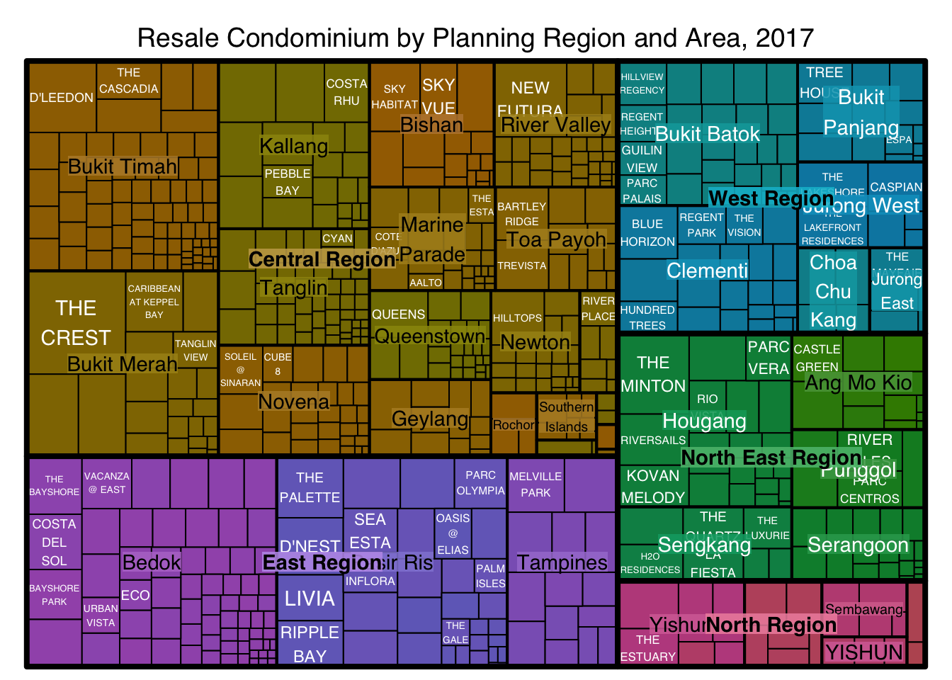
Warning
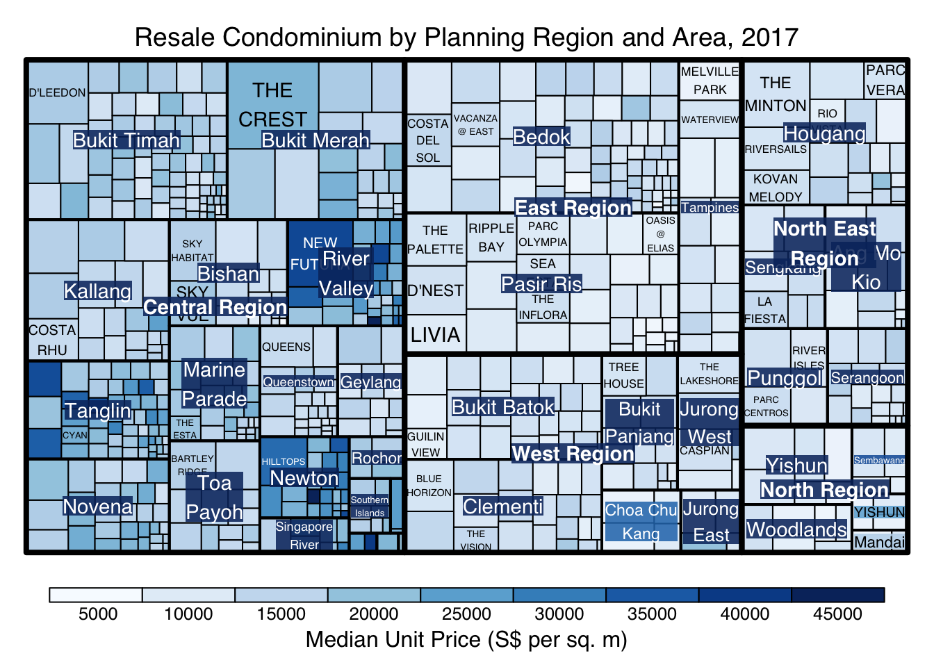
The treemap above was wrongly coloured. For a correctly designed treemap, the colours of the rectagles should be in different intensity showing, in our case, median unit prices.
For treemap(), vColor is used in combination with the argument type to determine the colours of the rectangles. Without defining type, like the code chunk above, treemap() assumes type = index, in our case, the hierarchy of planning areas.
4.3 Work with vColor and type arguments
In the code below, type argument is defined as “value”.
Show the code
treemap(realis2018_selected,
        index=c("Planning Region", "Planning Area", "Project Name"),
        vSize="Total Unit Sold",
        vColor="Median Unit Price ($ psm)",
        type = "value",
        title="Resale Condominium by Planning Region and Area, 2017",
        title.legend = "Median Unit Price (S$ per sq. m)"
        )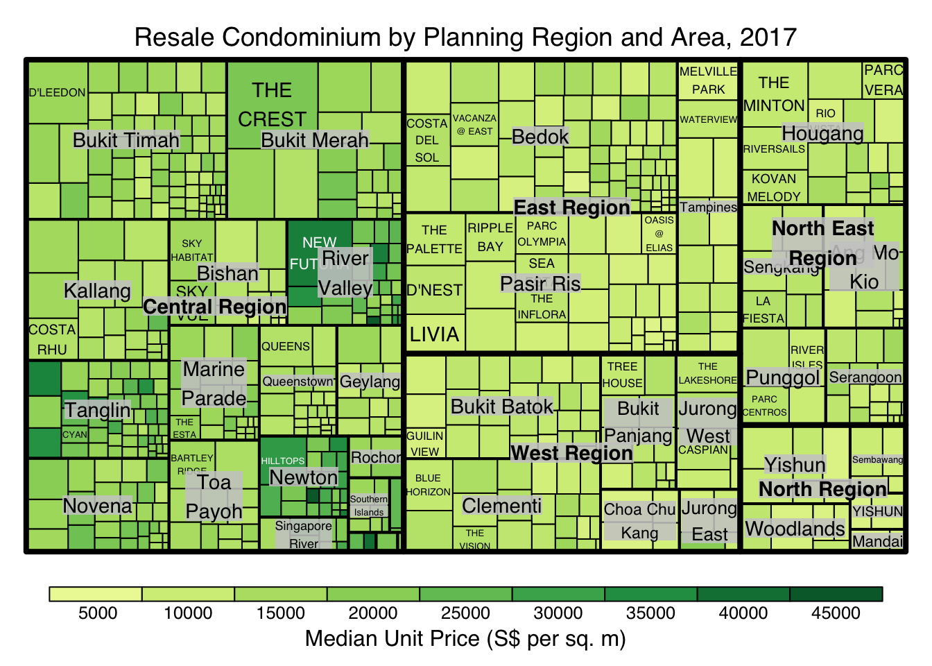
Learning from the code
The rectangles are coloured with different intensity of green, reflecting their respective median unit prices.
The legend reveals that the values are binned into ten bins, i.e. 0-5,000, 5,000-10,000, etc. with an equal interval of 5,000.
4.4 Colours in treemap package
There are two arguments that determine the mapping to color palettes: mapping and palette.
The only difference between “value” and “manual” is the default value for mapping.
The “value” treemap considers palette to be a diverging color palette (say ColorBrewer’s “RdYlBu”), and maps it in such a way that: - 0 corresponds to the middle color (typically white or yellow) - -max(abs(values)) to the left-end color - max(abs(values)) to the right-end color.
The “manual” treemap simply maps - min(values) to the left-end color - max(values) to the right-end color - mean(range(values)) to the middle color.
Show the code
treemap(realis2018_selected,
        index=c("Planning Region", "Planning Area", "Project Name"),
        vSize="Total Unit Sold",
        vColor="Median Unit Price ($ psm)",
        type="value",
        palette="RdYlBu",
        title="Resale Condominium by Planning Region and Area, 2017",
        title.legend = "Median Unit Price (S$ per sq. m)"
        )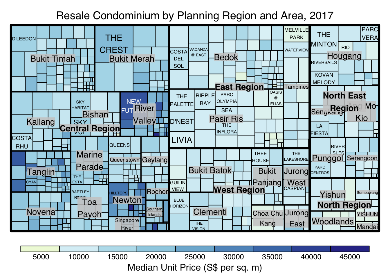
Learning from the code
Although the colour palette used is RdYlBu but there are no red rectangles in the treemap above. This is because all the median unit prices are positive.
The reason why we see only 5000 to 45000 in the legend is because the range argument is by default c(min(values, max(values)) with some pretty rounding.
The “manual” type does not interpret the values as the “value” type does. Instead, the value range is mapped linearly to the colour palette.
Show the code
treemap(realis2018_selected,
        index=c("Planning Region", "Planning Area", "Project Name"),
        vSize="Total Unit Sold",
        vColor="Median Unit Price ($ psm)",
        type="manual",
        palette="RdYlBu",
        title="Resale Condominium by Planning Region and Area, 2017",
        title.legend = "Median Unit Price (S$ per sq. m)"
        )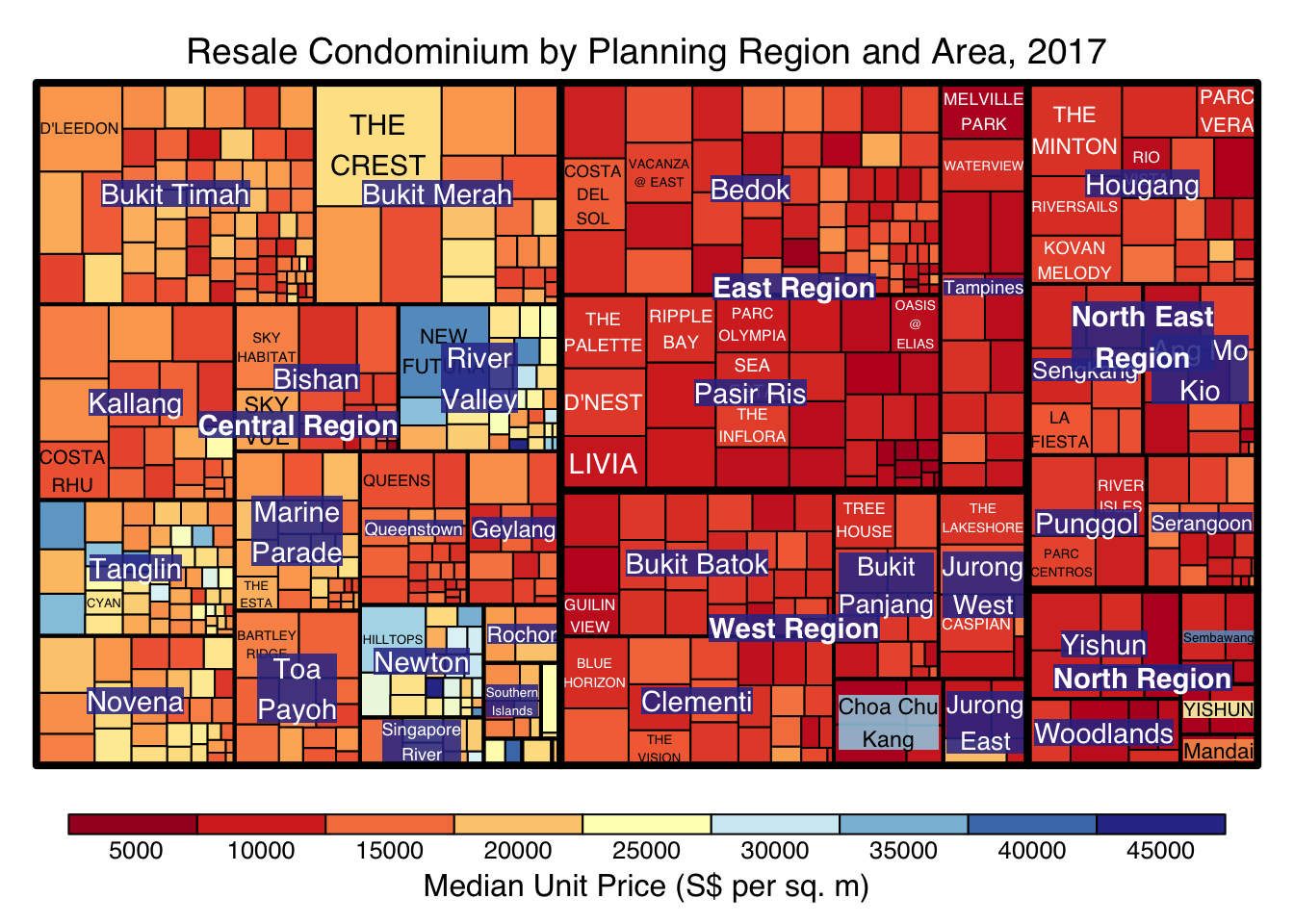
Learning from the code
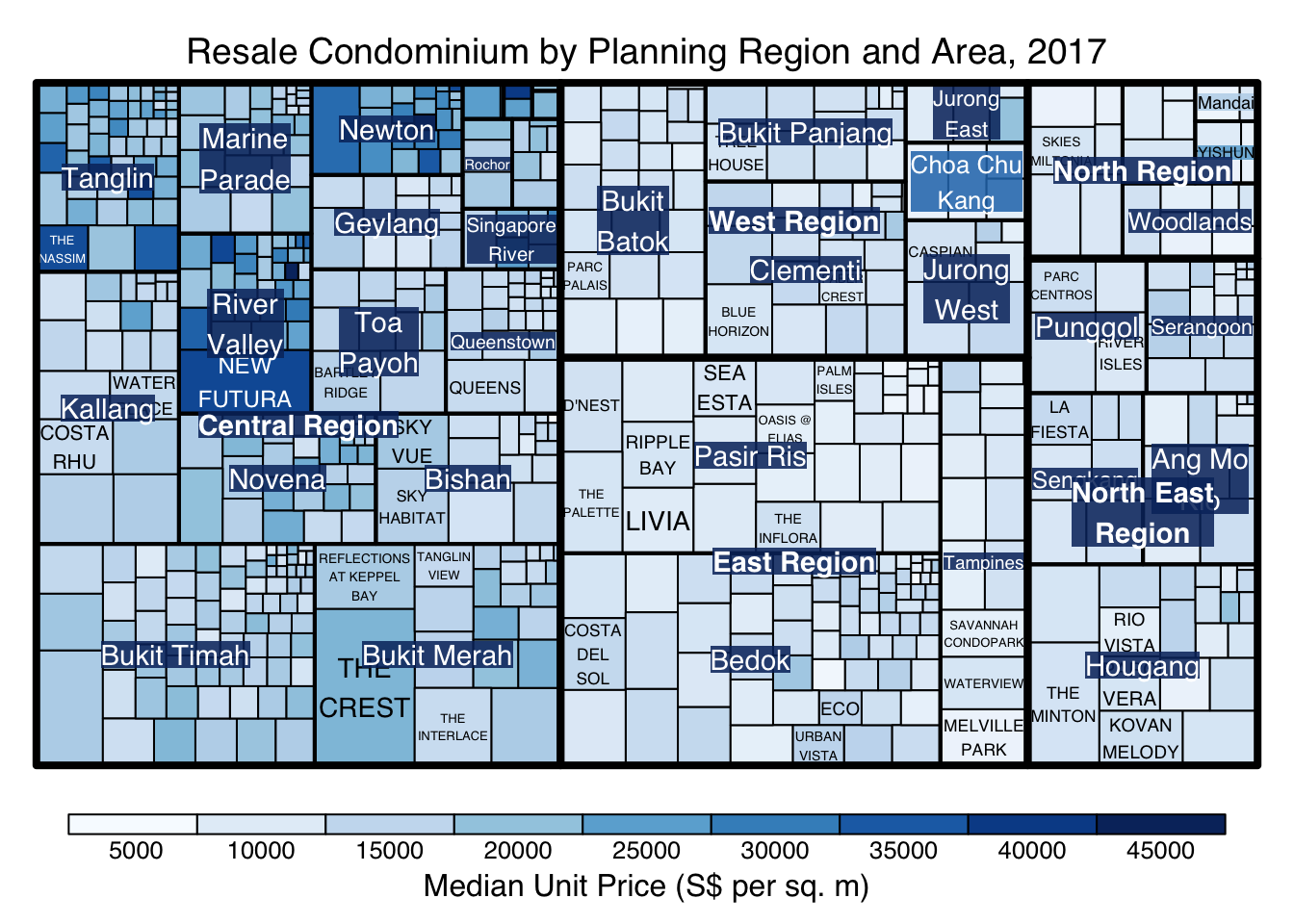
The colour scheme used is very copnfusing. This is because mapping = (min(values), mean(range(values)), max(values)).
It is not wise to use diverging colour palette such as RdYlBu if the values are all positive or negative ::: goals-container
To overcome this, a single color palette should be used, such as
Blues.
Show the code
treemap(realis2018_selected,
        index=c("Planning Region", "Planning Area", "Project Name"),
        vSize="Total Unit Sold",
        vColor="Median Unit Price ($ psm)",
        type="manual",
        palette="Blues",
        title="Resale Condominium by Planning Region and Area, 2017",
        title.legend = "Median Unit Price (S$ per sq. m)"
        )
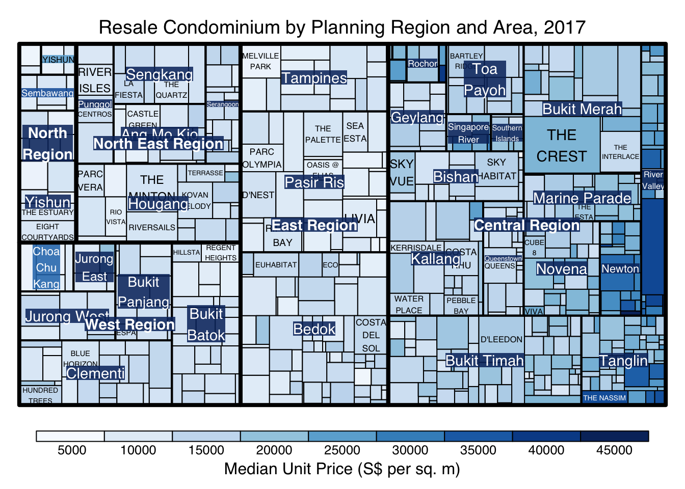
4.7 Treemap layout
reemap() supports two popular treemap layouts, namely: squarified and pivotSize. The default is pivotSize.
The squarified treemap algorithm (Bruls et al., 2000) produces good aspect ratios, but ignores the sorting order of the rectangles (sortID). The ordered treemap, pivot-by-size, algorithm (Bederson et al., 2002) takes the sorting order (sortID) into account while aspect ratios are still acceptable.
The code below plots a squarified treemap by changing the algorithm argument.
Show the code
treemap(realis2018_selected,
        index=c("Planning Region", "Planning Area", "Project Name"),
        vSize="Total Unit Sold",
        vColor="Median Unit Price ($ psm)",
        type="manual",
        palette="Blues",
        algorithm = "squarified",
        title="Resale Condominium by Planning Region and Area, 2017",
        title.legend = "Median Unit Price (S$ per sq. m)"
        )
When “pivotSize” algorithm is used, sortID argument can be used to dertemine the order in which the rectangles are placed from top left to bottom right.
Show the code
treemap(realis2018_selected,
        index=c("Planning Region", "Planning Area", "Project Name"),
        vSize="Total Unit Sold",
        vColor="Median Unit Price ($ psm)",
        type="manual",
        palette="Blues",
        algorithm = "pivotSize",
        sortID = "Median Transacted Price",
        title="Resale Condominium by Planning Region and Area, 2017",
        title.legend = "Median Unit Price (S$ per sq. m)"
        )
5 Design Treemap Using treemapify Package
treemapify is a R package specially developed to draw treemaps in ggplot2. We will learn how to design treemps closely resembling treemaps from previous section by using treemapify.
Resources: - Introduction to “treemapify” - user guide.
5.1 Design a basic treemap
Show the code
ggplot(data=realis2018_selected,
       aes(area = `Total Unit Sold`,
           fill = `Median Unit Price ($ psm)`),
       layout = "scol",
       start = "bottomleft") +
  geom_treemap() +
  scale_fill_gradient(low = "light blue", high = "blue") +
  theme(
      plot.title = element_text(hjust=0, family = "Bold"),
      plot.background = element_rect(fill = "#f1f4f5", color = "#f1f4f5"),
      legend.background = element_rect(fill="#f1f4f5"),
panel.background = element_rect(fill="#f1f4f5")) 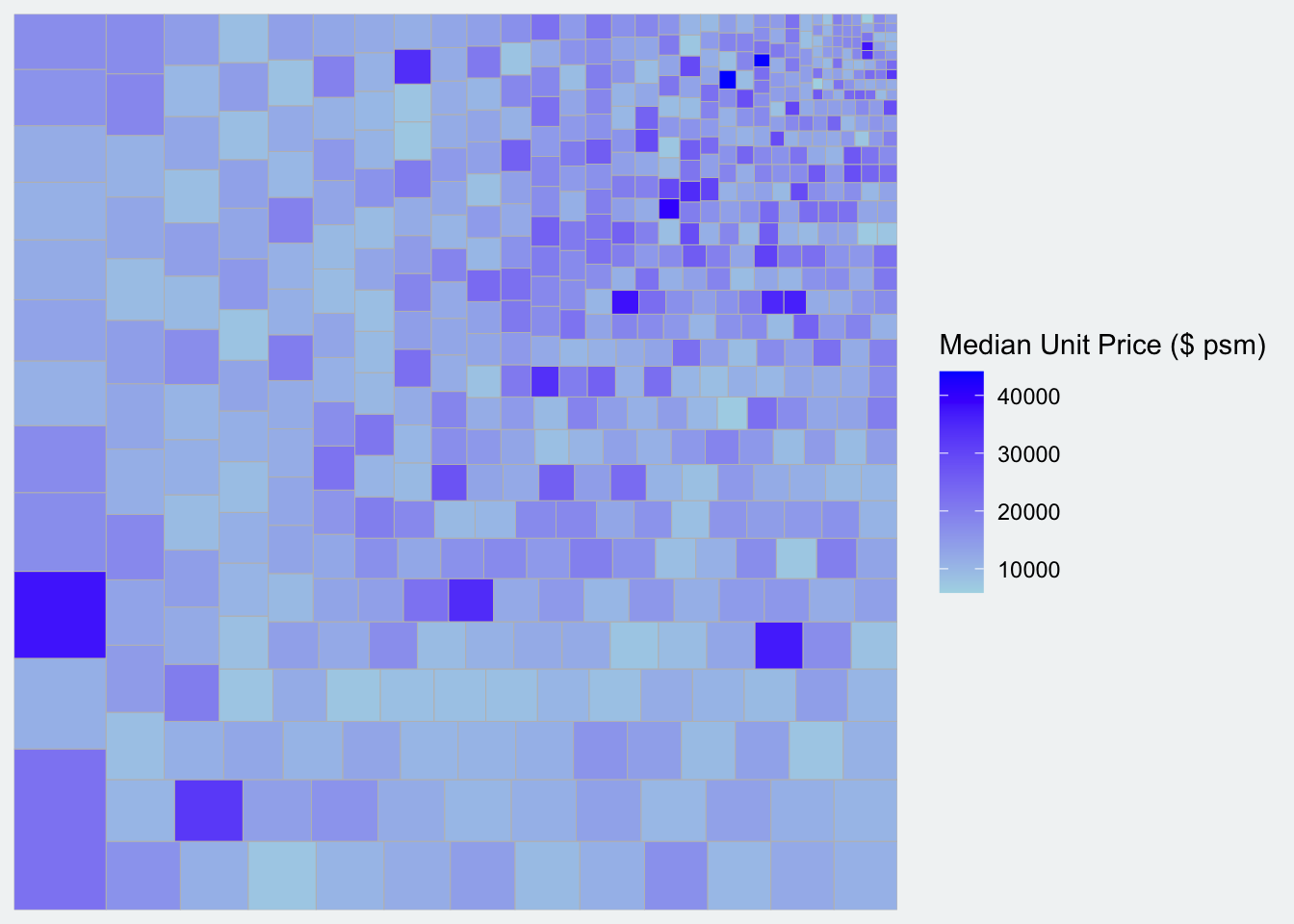
5.2 Define hierarchy
Show the code
ggplot(data=realis2018_selected,
       aes(area = `Total Unit Sold`,
           fill = `Median Unit Price ($ psm)`,
           subgroup = `Planning Region`),
       start = "topleft") +
  geom_treemap() +
  theme(
      plot.title = element_text(hjust=0, family = "Bold"),
      plot.background = element_rect(fill = "#f1f4f5", color = "#f1f4f5"),
      legend.background = element_rect(fill="#f1f4f5"),
panel.background = element_rect(fill="#f1f4f5")) 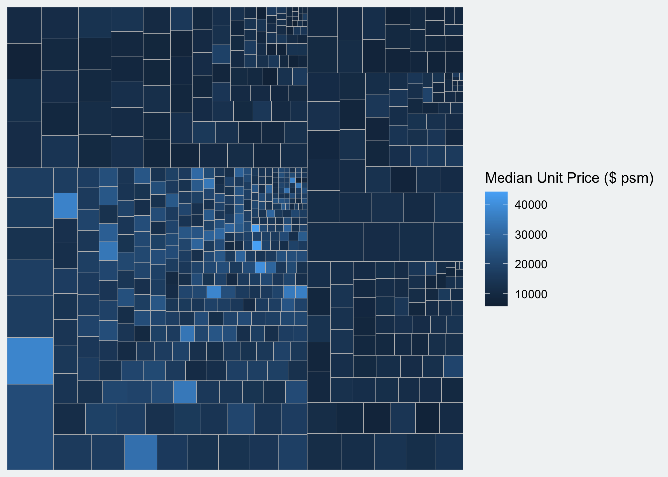
Show the code
ggplot(data=realis2018_selected,
       aes(area = `Total Unit Sold`,
           fill = `Median Unit Price ($ psm)`,
           subgroup = `Planning Region`,
           subgroup2 = `Planning Area`)) +  #added as subgroup2
  geom_treemap()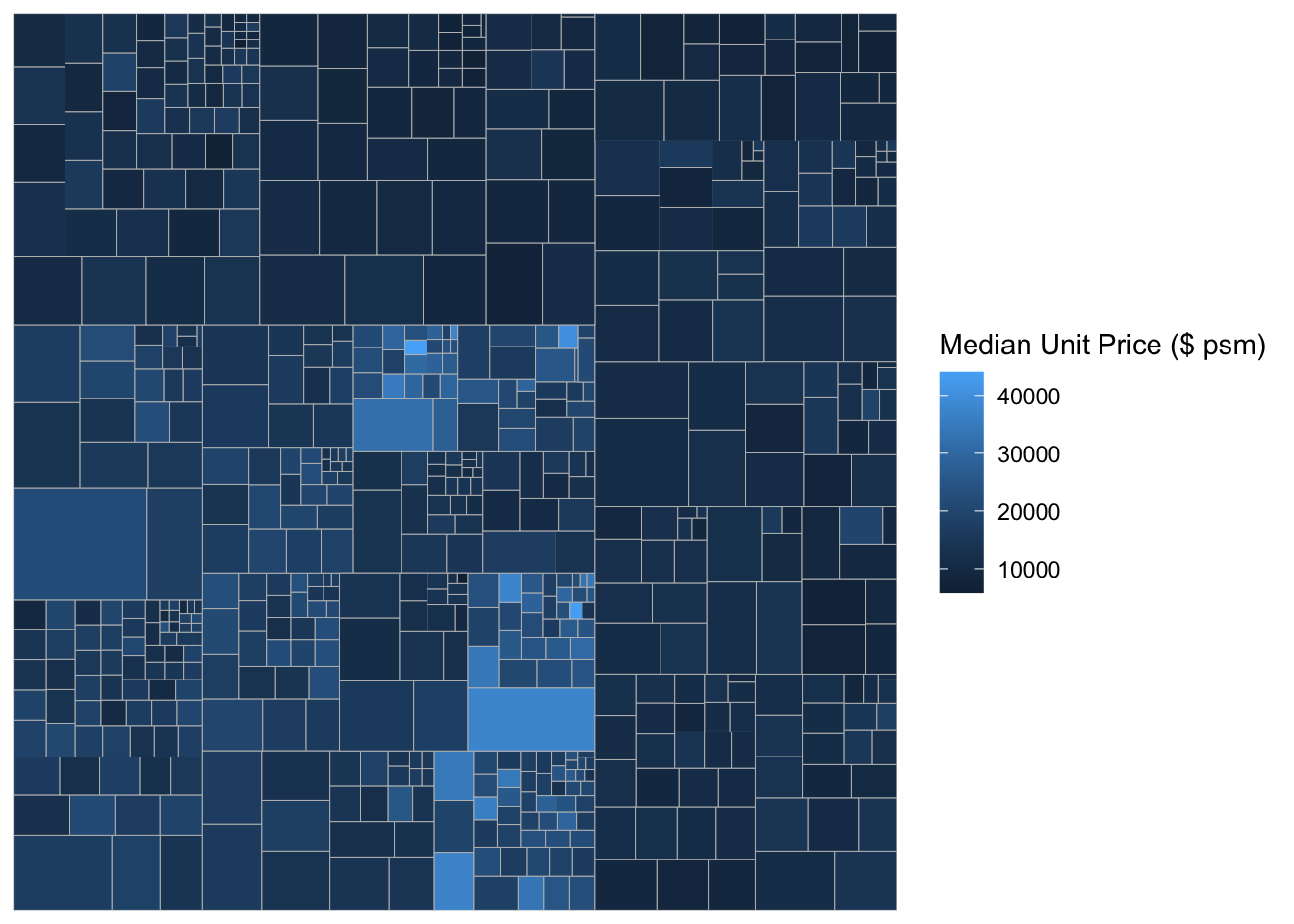
Show the code
ggplot(data=realis2018_selected,
       aes(area = `Total Unit Sold`,
           fill = `Median Unit Price ($ psm)`,
           subgroup = `Planning Region`,
           subgroup2 = `Planning Area`)) +
  geom_treemap() +
  geom_treemap_subgroup2_border(colour = "pink", #add lines
                                size = 2) +
  geom_treemap_subgroup_border(colour = "#BB993E")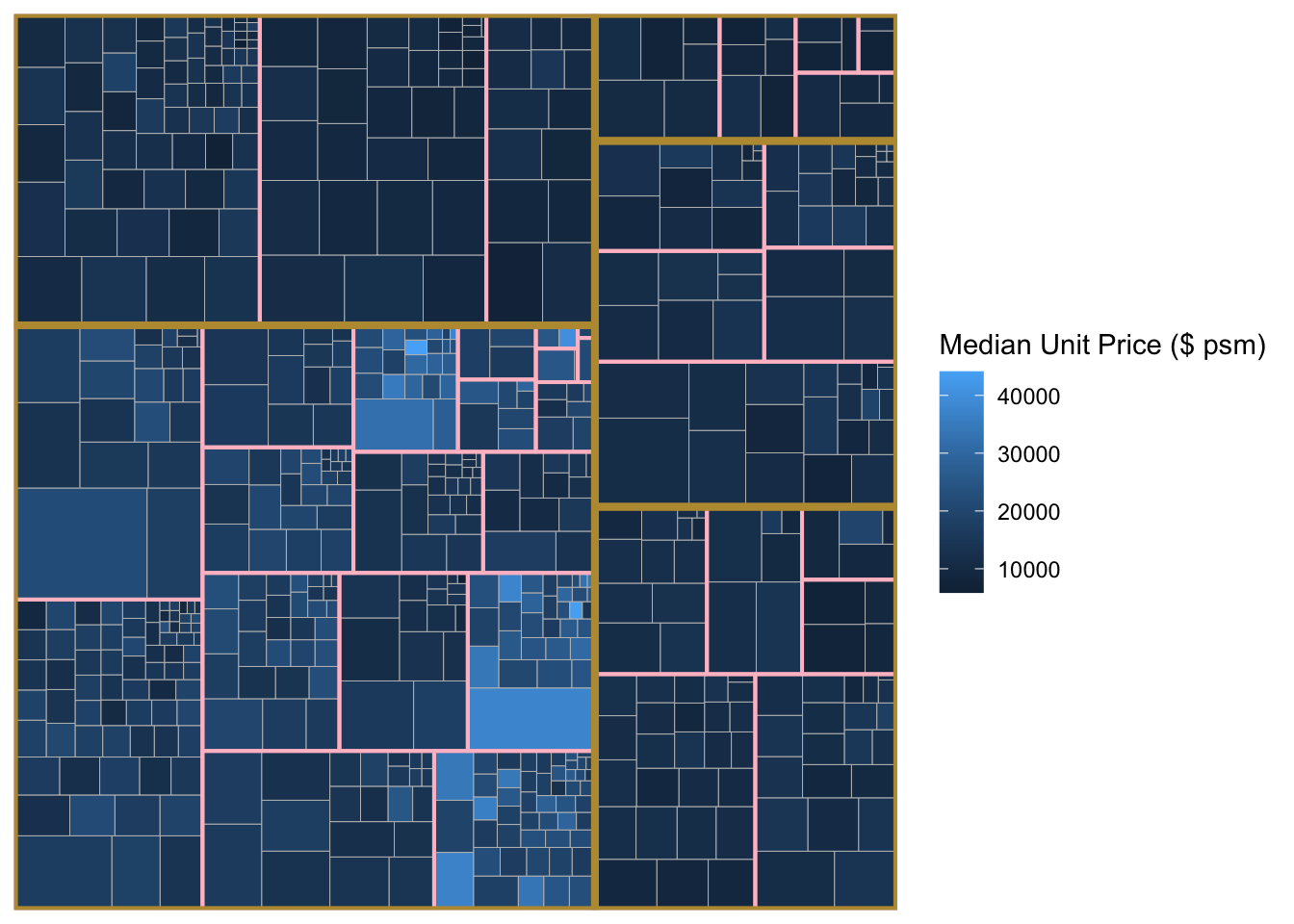
6 Design Interactive Treemap using d3treeR
6.1 Install d3treeR package
Step 1. Install devtool package
install.packages("devtools")Step 2. Load devtool library and install the package found in GitHub.
library(devtools)
install_github("timelyportfolio/d3treeR")
promises (1.3.2 -> 1.3.3 ) [CRAN]
utf8 (1.2.5 -> 1.2.6 ) [CRAN]
tibble (3.2.1 -> 3.3.0 ) [CRAN]
evaluate (1.0.3 -> 1.0.4 ) [CRAN]
data.table (1.17.0 -> 1.17.6) [CRAN]
gridSVG (NA -> 1.7-5 ) [CRAN]
data.tree (NA -> 1.1.0 ) [CRAN]
The downloaded binary packages are in
    /var/folders/nr/x4l8hvc562g81px_9hrd30_r0000gn/T//Rtmpr3cmx9/downloaded_packages
── R CMD build ─────────────────────────────────────────────────────────────────
* checking for file ‘/private/var/folders/nr/x4l8hvc562g81px_9hrd30_r0000gn/T/Rtmpr3cmx9/remotes176847c0c2d21/d3treeR-d3treeR-ebb833d/DESCRIPTION’ ... OK
* preparing ‘d3treeR’:
* checking DESCRIPTION meta-information ... OK
* checking for LF line-endings in source and make files and shell scripts
* checking for empty or unneeded directories
Omitted ‘LazyData’ from DESCRIPTION
* building ‘d3treeR_0.1.tar.gz’
force = TRUEStep 3. Launch d3treeR package
library(d3treeR)6.2 Design an interactive treemap
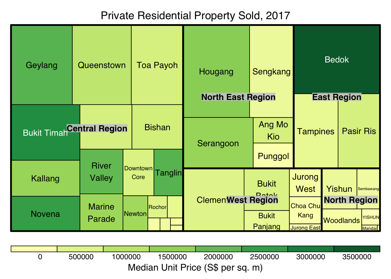
6.2.1 treemap() Base treemap
Step 1. treemap() is used to build a treemap by using selected variables in condominium data.frame. The treemap created is save as object called tm.
Show the code
tm <- treemap(realis2018_summarised,
        index=c("Planning Region", "Planning Area"),
        vSize="Total Unit Sold",
        vColor="Median Unit Price ($ psm)",
        type="value",
        title="Private Residential Property Sold, 2017",
        title.legend = "Median Unit Price (S$ per sq. m)"
        )
6.2.2 d3tree() Interactive treemap
d3tree(tm,rootname = "Singapore")